Stitched Panorama using OpenCV

            It is an interesting project to take a panorama view of a landscape giving the viewer a more immersive experience and a broader perspective of the surroundings.

A panoramic photo, made from multiple shots merged together, can be far more impressive than a single photo taken with a wide-angle lens. The OpenCV provides a set of open libraries of computer vision which can help detect same features from two different images and apply the image transformation homography to stitch the adjacent images together.

            In this project, several photos of the landscape of the Yosemite National Park will be stitched together using the computer vision technique.

There are five steps to form a panorama image:

• Find Keypoints and Descriptors for both images.
• Find Corresponding points by matching their Descriptors.
• Align second image with respect to first image using Homography.
• Warp the second image using Perspective Transformation.
• Combine the first image with the warped image to get the Panorama.

Step 1. Identify key features in each image

            Identify interesting stable points in an image using the ORB feature detector.

The ORB detector has the full name "Oriented FAST and Rotated BRIEF", a fusion of FAST keypoint detector and BRIEF descriptor

            The FAST keypoint detector identifies points on the image that are stable under image transformations like translation (shift), scale (increase / decrease in size), and rotation. The locator finds the (𝑥,𝑦) coordinates of such points. The FAST keypoint detector only identifies the location of interesting points.

            The BRIEF descriptor that uses binary strings to represent images. It encodes the appearance of the point so that we can distinguish one feature point from the other. The descriptor evaluated at a feature point is simply an array of numbers. Ideally, the same physical point in two images should have the same descriptor.

Reference: https://docs.opencv.org/4.x/d1/d89/tutorial_py_orb.html

(a) Convert the BGR image to a Gray image

im1Gray = cv2.cvtColor(im1, cv2.COLOR_BGR2GRAY)
im2Gray = cv2.cvtColor(im2, cv2.COLOR_BGR2GRAY)

(b) Use ORB detector to compute the Keypoints and Descriptors.

MAX_FEATURES = 5000
GOOD_MATCH_PERCENT = 0.01

orb = cv2.ORB_create(MAX_FEATURES)
keypoints1, descriptors1 = orb.detectAndCompute(im1Gray, None)
keypoints2, descriptors2 = orb.detectAndCompute(im2Gray, None)

(c) Use drawKeypoints to visualize the keypoints in one image

im1Keypoints = np.array([ ])
im1Keypoints = cv2.drawKeypoints(im1, keypoints1, im1Keypoints, color=(0,0,255),flags=0)

Step 2. Find Matching Points

            The matching algorithm DescriptorMatcher is to find the corresponding features (matching scores) in two images by comparing the descriptor of each feature in two images to conclude a list of match points. The hamming distance is used as a measure of similarity.

The Descriptor Matcher object ( matcher ) takes in two arrays of descriptors. The first argument is named queryDescriptor and second is named trainDescriptor.

The value GOOD_MATCH_PERCENT define the top portion of the found matches. The GOOD_MATCH_PERCENT shall be as low as possible to minimize the mismatching as long as it provides enough information for homography.

The output ( matches ) has the following attributes :

• matches.distance - Distance between descriptors. Should be lower for better match.
• matches.trainIdx - Index of the descriptor in train descriptors in image 2
• matches.queryIdx - Index of the descriptor in query descriptors in image 1
• matches.imgIdx - Index of the train image.

To simplify things, the queryIdx corresponds to points in image1 and trainIdx corresponds to points in image2. We will create two lists - points1 and points2 from the matching points which will serve as the final set of correspoding points to be used in the findHomography function.

Reference: https://docs.opencv.org/3.4/db/d39/classcv_1_1DescriptorMatcher.html

# Match features.
matcher = cv2.DescriptorMatcher_create(
                cv2.DESCRIPTOR_MATCHER_BRUTEFORCE_HAMMING)
matches = matcher.match(descriptors1, descriptors2, None)

# Sort matches by score
matches.sort(key=lambda x: x.distance, reverse=False)

# Remove not so good matches
numGoodMatches = int(len(matches) * GOOD_MATCH_PERCENT)
matches = matches[:numGoodMatches]

# Draw top matches
imMatches = cv2.drawMatches(im1, keypoints1,
                            im2, keypoints2, 
                            matches, None)

<matplotlib.image.AxesImage at 0x1e51e9a62b0>

Step 3. Image Alignment using Homography

            Homography is used to relate two images of a planar surface. The findHomography method utilizes a robust estimation technique called Random Sample Consensus (RANSAC) which produces the right result even in the presence of large number of bad matches.

X1 = H * X2

The point X1 is the same point (X2) in a different plane. H is their homography matrix.

The input of the findHomography method is the matching index from the descriptors.
The output of the findHomography method is a transformation matrix and a mask.
A mask of both inliers (1) (good points for a pattern) and outliers (0) (bad points).

Reference:
https://docs.opencv.org/4.x/d9/d0c/group__calib3d.html#ga4abc2ece9fab9398f2e560d53c8c9780

points1 = np.zeros((len(matches), 2), dtype=np.float32)
points2 = np.zeros((len(matches), 2), dtype=np.float32)

for i, match in enumerate(matches):
    points1[i, :] = keypoints1[match.queryIdx].pt
    points2[i, :] = keypoints2[match.trainIdx].pt

# Find homography
h1, mask = cv2.findHomography(points2, points1, cv2.RANSAC)

Step 4. Map images using warpPerspective

The warpPerspective function uses the transformation matrix to tranform all pixels in one image onto the other image's plane.
The perspective transformation is associated with the change in the viewpoint. It preserves collinearity and incidence.

Reference:
https://docs.opencv.org/4.x/da/d54/group__imgproc__transform.html#gaf73673a7e8e18ec6963e3774e6a94b87

# Use homography
im1Height, im1Width, channels = im1.shape
im2Height, im2Width, channels = im2.shape

im2Aligned = cv2.warpPerspective(im2, h1, 
                            (im2Width + im1Width, max(im1Height,im2Height)))

<matplotlib.image.AxesImage at 0x1e51e9c6370>

Step 5. Stitch images

The final image takes the transformed image2, which has the width of image 1 plus image 2. And superimpose image 1 on this new image plane.

# Stitch Image 1 with aligned image 2
stitchedImage = np.copy(im2Aligned)
stitchedImage[0:im1Height,0:im1Width] = im1

<matplotlib.image.AxesImage at 0x1e51aa624f0>

Trim the black edge before next stitching

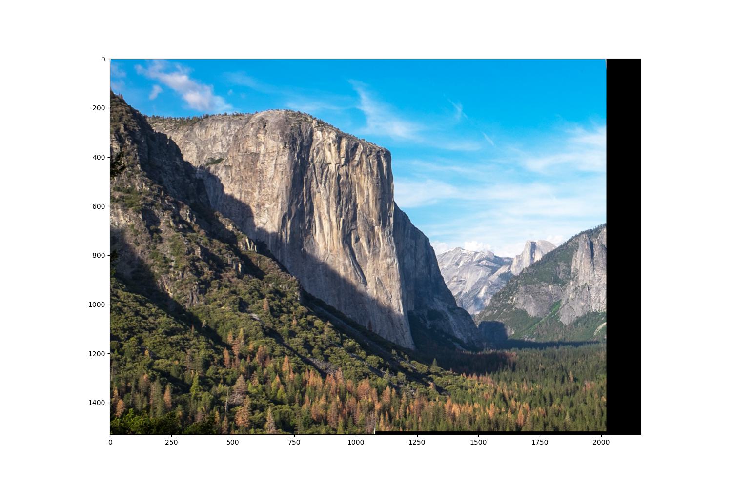
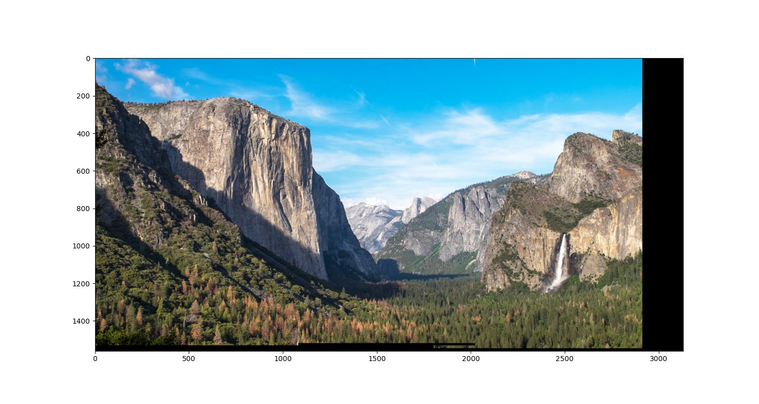
The image above shows an excellent job of stitching two adjacent images. Before the next iteration of stitching another image on the right, trim the black edge of the output image first.

Second iteration

Align another images on the right.

Keypoints identification

<matplotlib.image.AxesImage at 0x1e51e9f70d0>

<matplotlib.image.AxesImage at 0x1e51e3bf7f0>

Third iteration

Align another image on the right.

Keypoints identification

<matplotlib.image.AxesImage at 0x1e51e63e700>

Transformation matrix comparison

The transformation of these three iterations of adding one new image on the right has shown the different 8 degree-of-freedom transformation (rotation, translation, scaling and distortion) each new image is warped to align.

Homography matrix h1
[[ 9.99969815e-01  2.52185124e-05  9.40001998e+02]
 [-4.93834659e-05  1.00005308e+00 -1.20234866e+01]
 [-5.34637067e-08  2.81264120e-08  1.00000000e+00]]
 
Homography matrix h2 
[[ 9.99005637e-01  1.90341980e-04  1.79998927e+03]
 [-2.28665437e-04  1.00005913e+00 -1.49861139e+01]
 [-5.08172904e-07  9.44819979e-08  1.00000000e+00]]

Homography matrix h3
[[1.07542304e+00 7.12265257e-03 2.73064794e+03]
 [1.07707507e-02 1.00737430e+00 1.24853914e+01]
 [2.65999072e-05 2.53025908e-06 1.00000000e+00]] 
 

End of File