The IsolationForest ‘isolates’ observations by randomly selecting a feature and then randomly selecting a split value between the maximum and minimum values of the selected feature.
Since recursive partitioning can be represented by a tree structure, the number of splittings required to isolate a sample is equivalent to the path length from the root node to the terminating node.
This path length, averaged over a forest of such random trees, is a measure of normality and our decision function.
Random partitioning produces noticeably shorter paths for anomalies. Hence, when a forest of random trees collectively produce shorter path lengths for particular samples, they are highly likely to be anomalies.
Isolation Forest Algorithm returns the anomaly score of each sample.
Reference:
https://scikit-learn.org/stable/modules/generated/sklearn.ensemble.IsolationForest.html
The Skoltech Anomaly Benchmark (SKAB) datasets are a collection of multivariate time-series data specifically designed to evaluate the performance of anomaly detection algorithms. The data comes from sensors installed on a testbed that simulates the flow of water in a closed circuit.
The multivariate time-series include sensor data such as current, temperature, voltage, accelerometer1RMS, accelerometer2RMS, volumeflowrateRMS, pressure, and thermocouple reading. It can be downloaded as a csv file.
Read the csv content into a dataframe:
import pandas as pd
DF = pd.read_csv("SKABt.csv", sep=";", decimal=",")
References:
Skoltech Anomaly Benchmark: https://www.kaggle.com/datasets/yuriykatser/skoltech-anomaly-benchmark-skab-teaser
(1) Convert the 'value' column to numeric and invalid parsing into "Nan".
DF["value"] = pd.to_numeric(DF["value"], errors="coerce")
(2) The 'id' column indicates the names of sensor modality. Divide the dataframe into subsets according to its 'id'. For example, currentDF collects current data.
currentDF=DF[DF['id']=='Current']
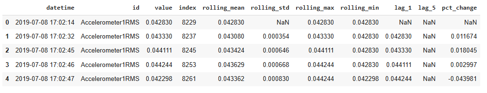
For each time series, the features include rolling and lag. Include the following data feature actions into one function, called "create_feature".
(1) Sort the group by 'datetime' to ensure chronological order
group = group.sort_values("datetime")
(2) Calculate rolling mean with a window of 10, minimum 1 period to avoid NaN
group["rolling_mean"] = group["value"].rolling(window=10, min_periods=1).mean()
(3) Calculate rolling standard deviation with a window of 10, minimum 1 period
group["rolling_std"] = group["value"].rolling(window=10, min_periods=1).std()
(4) Calculate rolling maximum with a window of 10, minimum 1 period
group["rolling_max"] = group["value"].rolling(window=10, min_periods=1).max()
(5) Calculate rolling minimum with a window of 10, minimum 1 period
group["rolling_min"] = group["value"].rolling(window=10, min_periods=1).min()
(6) Create lag features: value shifted by 1
group["lag_1"] = group["value"].shift(1)
(7) Create lag features: value shifted by 5
group["lag_5"] = group["value"].shift(5)
(8) Calculate the percentage change from the previous value
group["pct_change"] = group["value"].pct_change()
data=currentDF.copy()
PhyFeature="Current"
(1) Convert 'datetime' column to datetime object
data["datetime"] = pd.to_datetime(data["datetime"])
(2) Apply the 'create_features' function to each sensor modality group such as 'CurrentDF' data = data.groupby("id").apply(create_features).reset_index(drop=True)
The sample output is as follows:
(3) Make a list of feature column names
feature_cols =
["value", "rolling_mean", "rolling_std", "rolling_max",
"rolling_min", "lag_1", "lag_5", "pct_change", ]
(4) Replace infinite value with Nan
data[feature_cols] = data[feature_cols].replace([np.inf, -np.inf], np.nan)
(5) Forward fill NaN values to propagate the last valid observation forward.
Backward fill any remaining NaNs to ensure no missing values remain.
data[feature_cols] = data[feature_cols].fillna(method="ffill").fillna(method="bfill")
(6) Scale features to deal with outliers.
The RobustScaler in scikit-learn is a preprocessing technique used to scale features in a dataset, particularly useful when dealing with outliers. It removes the median and scales the data according to the Interquartile Range (IQR), which is the range between the 25th and 75th percentiles.
from sklearn.preprocessing import RobustScaler
scaler = RobustScaler()
X = scaler.fit_transform(data[feature_cols])
For. example, the 8 feature columns are transformed as follows:
X[0:5]=array([
[ 1.95416708, 1.96953091, -0.99640656, 1.41601072, 2.86163419,
1.95251508, 1.93978204, 0.22560053],
[ 2.11998806, 2.05098164, -0.99640656, 1.55557416, 2.86163419,
1.95251508, 1.93978204, 0.22560053],
[ 2.37929891, 2.163047 , -0.18005362, 1.77382348, 2.86163419,
2.11819869, 1.93978204, 0.35767909],
[ 2.42314198, 2.22984746, -0.11846089, 1.81072406, 2.86163419,
2.37729472, 1.93978204, 0.0457178 ],
[ 1.77779989, 2.14313175, 0.33337906, 1.81072406, 2.64393319,
2.42110146, 1.93978204, -0.92816506]])
Reference:
https://scikit-learn.org/stable/modules/generated/sklearn.preprocessing.RobustScaler.html
For each series of the same feature, count the elements whose values exceeding 3 standard deviations. The output of the contamination function is a percentage of outlier to the total number of elements in the same series. For example, there are 80 outliers in a series of 6405 elements. The contamination proportion is 0.012. If there are 5 data series, further obtain the mean values of the five contamination proportion values as the final contamination rate.
Bound the contamination between 1% and 20%.
contamination = estimate_contamination(X)
contamination = min(max(contamination, 0.01), 0.2)
def estimate_contamination(X):
    outlier_proportions = []
    for feature_idx in range(X.shape[1]):
        # Extract all values for the current feature
        feature_values = X[:, feature_idx]

        # Calculate mean and standard deviation of the feature
        mean = np.mean(feature_values)
        std = np.std(feature_values)

        # Count the number of outliers beyond 3 standard deviations from the mean
        outliers = np.sum(np.abs(feature_values - mean) > 3 * std)

        # Calculate the proportion of outliers in the current feature
        outlier_proportions.append(outliers / len(feature_values))

    # Return the average contamination rate across all features
    return np.mean(outlier_proportions)
For each set of the same sensor modality data, split the dataset into training and validation sets with an 80-20 split. random_state=42 ensures reproducibility. Each sensor set will have its own IsolationForest model.
from sklearn.model_selection import train_test_split
X_train, X_test = train_test_split(X, test_size=0.2, random_state=42)
Reference:
https://scikit-learn.org/stable/modules/generated/sklearn.model_selection.train_test_split.html
Set up the contamination rate to be the average outlier proportion, calculated above.
from sklearn.ensemble import IsolationForest
IsoForest = IsolationForest(contamination=contamination, random_state=42)
Reference:
https://scikit-learn.org/stable/modules/generated/sklearn.ensemble.IsolationForest.html
IsoForest.fit(X_train)
In the prediction, value 1 indicates normal. Otherwise, anomaly.
test_prediction=IsoForest.predict(X_test)
Organize the labels to be (1, normal) and (0, anomaly)
test_prediction = [1 if x == 1 else 0 for x in test_prediction]
If the test set has ground truth labels, then the F1 score can be calculated to evaluate the training model performance.
The F1 score is a machine learning evaluation metric that calculates the harmonic mean of precision and recall, where an F1 score reaches its best value at 1 and worst score at 0. Its formula is
from sklearn.metrics import f1_score
f1 = f1_score(test_groundtruth, test_prediction)
Reference:
https://scikit-learn.org/stable/modules/generated/sklearn.metrics.f1_score.html
https://scikit-learn.org/stable/auto_examples/model_selection/plot_precision_recall.html
(1) Generate the prediction labels for the entire data series.
data["anomaly"] = IsoForest.predict(X)
(2) Map the predictions to binary labels: 0 for normal instances, 1 for anomalies.
data["anomaly"] = data["anomaly"].map({1: 0, -1: 1}) # Convert to 0 (normal) and 1 (anomaly)
(3) Record the location of the anomaly.
(4) Visualize the timing of the anomaly by plotting 'datetime' versus 'data'.
PhyFeature="Current"

a = data.loc[data['anomaly'] == 1] #anomaly subset
_ = plt.figure(figsize=(18,6))
_ = plt.plot( data['datetime'], data['value'], color='blue', label='Raw data')
_ = plt.plot(  a['datetime'], a['value'], linestyle='none', marker='X', color='red', markersize=2, label='Anomaly')
_ = plt.xlabel('Schedule')
_ = plt.ylabel(PhyFeature+' Reading')
_ = plt.title(PhyFeature+' Anomalies')
_ = plt.legend(loc='best')
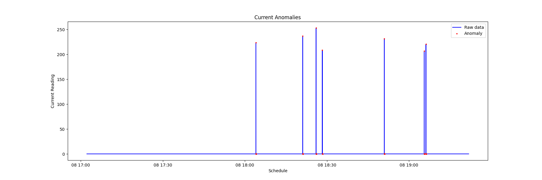


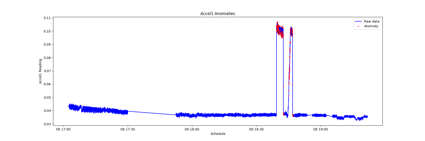
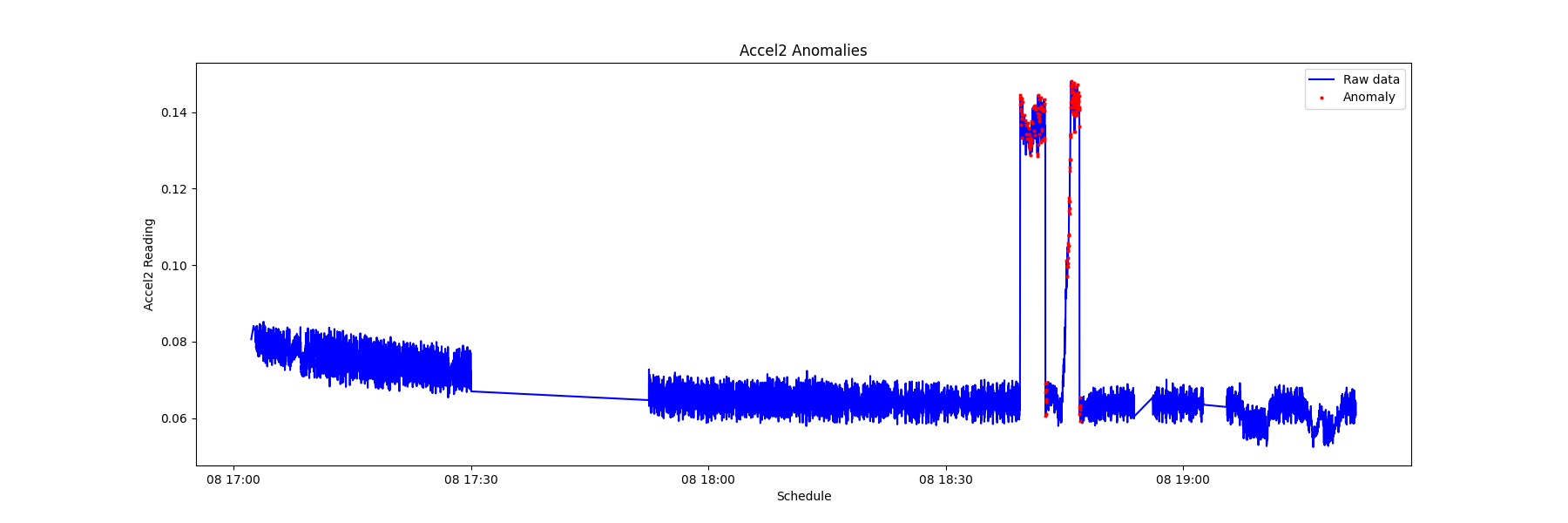
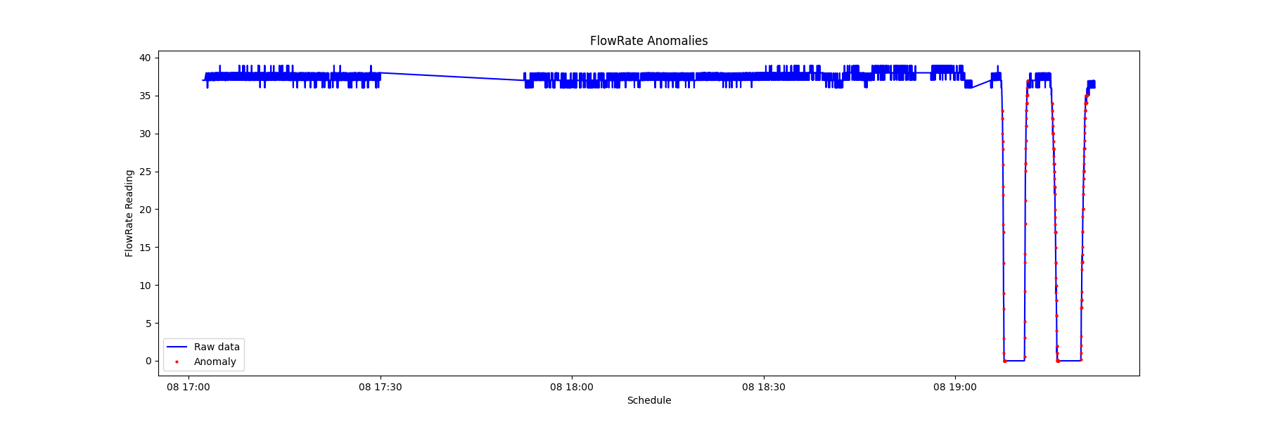

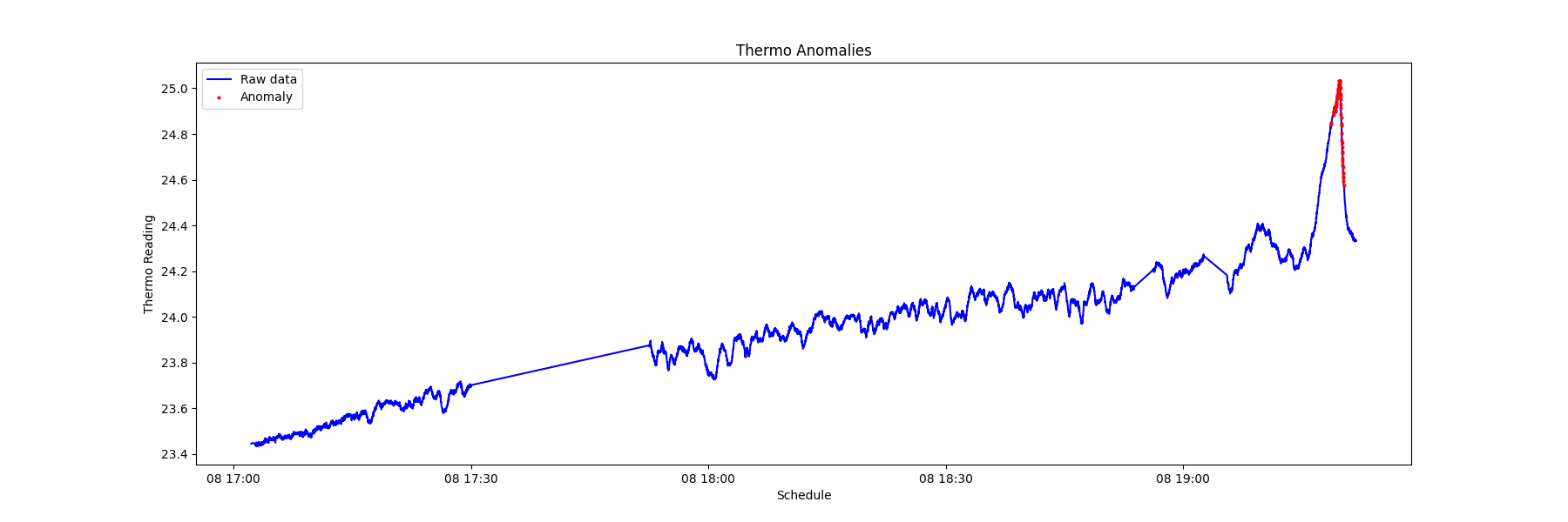
By recording the timing of the anomalies of various sensors, it is possible to view the sequence of modality anomalies and potentially catch the system failure from an early sign of specific sensor data signatures.
CurrentAnom=data.loc[data['anomaly']==1]
From the chart below, it is observed that the electrical current anomaly and the accelerometer anomaly can be used as the early warning of a system failure.
